By Eric Gregori
Senior Software Engineer
BDTI
This article was originally published at EE Times' Embedded.com Design Line. It is reprinted here with the permission of EE Times.
With the emergence of increasingly capable low-cost processors and image sensors, it’s becoming practical to incorporate computer vision capabilities into a wide range of embedded systems, enabling them to analyze their environments via image and video inputs.
Products like Microsoft’s Kinect game controller and Mobileye’s driver assistance systems are raising awareness of the incredible potential of embedded vision technology. As a result, many embedded system designers are beginning to think about implementing embedded vision capabilities.
In this article, the second in a series, we introduce edge detection, one of the fundamental techniques of computer vision. Like many aspects of computer vision, edge detection sounds simple but turns out to be complex. We explore some of the common challenges and pitfalls associated with edge detection, and present techniques for addressing them. Then, after explaining edge detection from an algorithmic perspective, we show how to use OpenCV, a free open-source computer vision software component library, to quickly implement application software incorporating edge detection. For an overview of computer vision and OpenCV, read "Introduction to Embedded Vision and the OpenCV Library."
What is an "Edge" in Computer Vision?
Images, of course, are made up of individual points called pixels. In a grayscale image, the value of each pixel represents the intensity of the light captured when creating the image. An edge is defined as an area of significant change in the image intensity. Figure 1 below shows a grayscale image on the left, with its corresponding binary edge map on the right. If you look carefully, you will notice that the white lines in the edge map delineate the portions of the image separated by pixels of different intensity.
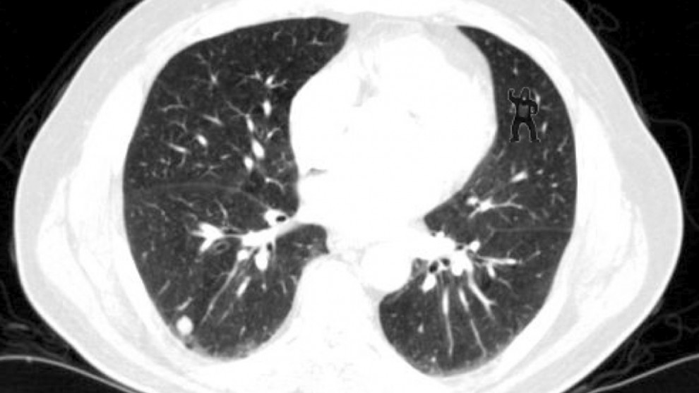
Figure 1. Grayscale image and its corresponding binary edge map
If you graph the values of a single row of pixels containing an edge, the strength of the edge is shown by slope of the line in the graph. We use the term "hard" to describe an edge with a large difference between nearby pixel values, and "soft" to describe small differences in close-proximity pixel values.
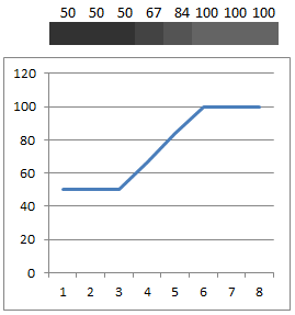
Figure 2. Grayscale soft edge
Figure 2 above and Figure 3 below represent eight pixels from two different parts of a grayscale image. The numeric value for each pixel is shown above an expanded view of the actual pixel. Figure 2 represents a "soft" edge while Figure 3 represents a "hard" edge.

Figure 3. Grayscale hard edge
How Edges are Used in Computer Vision
The goal of a computer vision application is to extract meaning from images. In general, this objective is first accomplished by finding relevant features in the images. Edges are one type of image feature.
For example, edges can be used to find the boundaries of objects in an image, in order to enable isolating those objects for further processing. This process is known as "segmentation." After an image is segmented, objects can be individually analyzed or discarded depending on what the application is trying to accomplish.
Unfortunately, in many applications, not all edges in an image actually represent separate objects, and not all objects are separated by clean edges. As mentioned earlier, edges are graded on a scale from no edge to "soft" edge, and finally to "hard" edge. Somewhere in the algorithm, a decision has to be made regarding whether a given edge is "hard" enough to be classified as a true edge versus, for example, just a small change in brightness due to lighting variation.
Finding Edges in an Image: The Canny Algorithm
Many algorithms exist for finding edges in an image. This example focuses on the Canny algorithm. Considered by many to be the best edge detector, the Canny algorithm was described in 1986 by John F. Canny of U.C. Berkeley. In his paper, "A Computational Approach to Edge Detection," Canny describes three criteria to evaluate the quality of an edge detection algorithm:
- Good detection: There should be a low probability of failing to mark real edge points, and a low probability of falsely marking non-edge points. This criterion corresponds to maximizing signal-to-noise ratio.
- Good localization: The points marked as edge points by the operator should be as close as possible to the center of the true edge.
- Only one response to a single edge: This criterion is implicitly also captured in the first one, since when there are two responses to the same edge, one of them must be considered false.
The algorithm achieves these criteria using multiple stages, as shown in Figure 4 below.
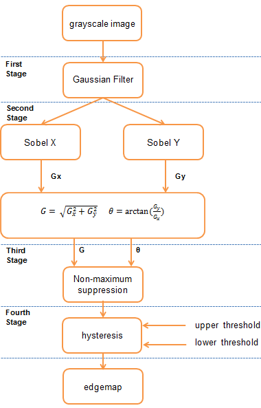
Figure 4. Block diagram of the Canny edge detection algorithm
First Stage: Gaussian Filter
In the first stage of the Canny edge detection algorithm, noise in the image is filtered out using a Gaussian filter. This step is referred to as image smoothing or blurring. The Gaussian filter removes the high frequency white noise (i.e. "popcorn noise") common with images collected from CMOS and CCD sensors, without significantly degrading the edges within the image.
The amount of blurring done by the Gaussian filter is controlled in part by the size of the filter kernel. As the filter kernel size increases, the amount of blur also increases. Too much blur will soften the edges to a point where they cannot be detected. Too little blur conversely will allow noise to pass through, which will be detected by the next stage as false edges. The series of images in Figure 5 below shows the result of applying a Gaussian filter to a grayscale image.
Figure 5a. Original image
Figure 5b. Gaussian filtered image: filter kernel size 3

Figure 5c. Gaussian filtered image: filter kernel size 5

Figure 5d. Gaussian filtered image: filter kernel size 7
Second Stage: Intensity Gradient
The second stage of the Canny edge detection algorithm calculates the intensity gradient of the image using a first derivative operator. Looking back at Figures 2 and 3, the intensity gradient corresponds to the slope of the line in the graph. The intensity gradient of an image reflects the strength of the edges in the image.
Strong edges have larger slopes and therefore have larger intensity gradients. The slope of a line can be calculated using a first derivative operator. The original Canny paper tested various first derivative operators; most modern Canny implementations (including the one in the OpenCV library) use the Sobel operator (Figure 6, below).

Figure 6. Vertical derivative of the image shown in Figure 5b, calculated using the Sobel operator
The Sobel operator separately returns the first derivative of the image in the horizontal and vertical directions. This process is done on every pixel in the image. The Sobel operator results in two images, with each pixel in the first image representing the horizontal derivative of the input image and each pixel in the second image representing the vertical derivative, as illustrated in Figure 6 above and Figure 7 below.

Figure 7. Horizontal derivative of the image shown in Figure 5b, calculated using the Sobel operator
To calculate the overall image gradient requires converting the horizontal and vertical scalar values to a vector value comprising a magnitude and an angle. Given horizontal and vertical scalars, the vector can be calculated using the equations in Figure 8 below.
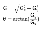
Figure 8. Converting the horizontal and vertical first derivative scalar values to a vector
The equations in Figure 8 are applied to each pixel, resulting in an image gradient such as the one shown in Figure 9 below.

Figure 9. Image gradient of the image shown in Figure 5b
Each pixel has a magnitude and angle value, although Figure 9 shows only the magnitude; the angle information is not included. Sharper edges have higher magnitudes.
Note how thick the edges in Figure 9 are. This is a by-product of the method that the Sobel operator uses to calculate the first derivative, which employs a group of pixels. The minimum number of pixels is nine, organized as a 3-pixel-by-3-pixel square cluster.
This 3×3 group of pixels is used to calculate the derivative of the single pixel in the center of the group. The group size is important because it has an effect both on the performance of the operator and on the number of computation operations required. In this case, a smaller operator creates the cleanest edges.
Third Stage: Non-Maximum Suppression
The next stage in the Canny algorithm thins the edges created by the Sobel operator, using a process known as non-maximum suppression. Non-maximum suppression removes all pixels that are not actually on the edge "ridge top," thereby refining the thick line into a thin line. Simply put, non-maximum suppression finds the peak of the cross section of the thick edge created by the Sobel operator. Figure 10 below shows a graph of a single row of pixels from an edge detected in Figure 9.
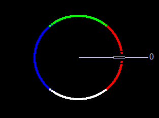
Figure 10. Thick edges caused by the Sobel operator
The non-maximum suppression method finds the peak of the edge by scanning across the edge using the angle data calculated by the Sobel operator, looking for a maximum magnitude. Any pixels less than the maximum magnitude are set to zero. The result is shown in Figure 11 below. Notice that the edges have been thinned, but they are still not perfect.
Figure 11. Thinned edge using non-maximum suppression
Fourth Stage: Hysteresis
The final stage of the Canny edge detector is referred to as hysteresis. In this stage, the detector uses high (T2) and low (T1) threshold values to filter out pixels in the gradient image left over from the previous stage that are not part of an edge.
The algorithm first finds a gradient in the image greater than T2. It then follows the gradient, marking each pixel that is greater than T1 as a definite edge. The algorithm requires a gradient greater than the high threshold to begin following the edge, but it will continue to follow the edge as long as the gradient stays above the low threshold.
Any pixels with gradients below T2 that are not connected to gradients above T1 are rejected as edges. This hysteresis helps to ensure that noisy edges are not broken up into multiple edge fragments.
Finding Edges in an Image Using OpenCV
OpenCV is an open-source software component library for computer vision application development, and a powerful tool for prototyping embedded vision algorithms. Originally released in 2000, it has been downloaded over 3.5 million times. The OpenCV library comprises more than 2,500 functions and contains dozens of valuable vision application examples. The library supports C, C++, and Python, and has been ported to Windows, Linux, Android, Mac OS X, and iOS.
The great thing about OpenCV is how much work it does for you behind the scenes. Some of the leading minds in the field have contributed to the OpenCV library, making it a very powerful tool. You can find the edges in a grayscale image using the OpenCV Canny() function described here (from the OpenCV documentation):
void Canny(InputArray image, OutputArray edges, double threshold1, double threshold2, int apertureSize=3, bool L2gradient=false)
|
image |
Single-channel 8-bit input image. |
|
edges |
Output edge map. It has the same size and type as image. |
|
threshold1 |
First threshold for the hysteresis procedure. |
|
threshold2 |
Second threshold for the hysteresis procedure. |
|
apertureSize |
Aperture size for the Sobel() operator. |
|
L2gradient |
Flag indicating method used to calculate magnitude of gradient. |
The input image must be a grayscale image. An example of how to convert a color image to a grayscale image will be discussed in detail later in this article. The output will also be a grayscale image with edges marked as 1 and non-edges marked as 0.
threshold1 and threshold2 are the upper (T1) and lower (T2) Canny thresholds used in the fourth (hysteresis) stage of the algorithm.
apertureSize sets the size of the Sobel operator used in stage two of the Canny algorithm. In the OpenCV implementation, the apertureSize size can be 3, 5, or 7, representing operator sizes of 3×3, 5×5, and 7×7, respectively.
The L2gradient flag determines the method used to calculate the magnitude when combining the horizontal and vertical Sobel results, as shown in Figure 8. For performance purposes, OpenCV offers a simplified form of the magnitude equation in Figure 8, eliminating the square root operation. The equation G = |Gx| + |Gy| gives a rough approximation to G = sqrt( Gx^2 + Gy^2 ) without requiring an expensive square root operation. Setting L2gradient false uses the faster G = |Gx| + |Gy| equation to calculate the magnitude.
OpenCV Canny Edge Detector Examples
Two easy-to-use tools have been created to help developers get up and running with OpenCV. The first tool, the BDTI OpenCV Executable Demo Package, is Microsoft Windows-based and allows you to experience OpenCV using just your mouse, with no programming required. The BDTI OpenCV Executable Demo Package includes various OpenCV examples that you can execute by simply double clicking on an icon.
All of the examples have sliders that allow you to alter each demonstrated computer vision algorithm by adjusting parameters with the mouse.
You can download the BDTI OpenCV Executable Demo Package here (free registration is required). BDTI has also developed an online user guide and tutorial video for the BDTI OpenCV Executable Demo Package.
The second tool, the BDTI Quick-Start OpenCV Kit, is for engineers who want to develop their own algorithms using OpenCV and who want to get started quickly. The included VMware virtual machine image is Ubuntu Linux-based and runs on a Windows machine using the free VMware Player. OpenCV, along with all the required packages and tools, have been preinstalled in the image so the user can be up in running in minutes, with no prior Linux experience required.
The image contains Eclipse and GCC for C/C++ development, pre-installed and configured with many OpenCV examples. Eclipse is a very common and easy to use graphical integrated development environment (IDE) that makes it easy to get OpenCV up and running. The BDTI Quick-Start OpenCV Kit is a full OpenCV installation, with source code included so you can configure the library to your own specific needs. The library is prebuilt with a documented configuration, making it easy to get up and running quickly.
You can download the BDTI Quick-Start OpenCV Kit here (free registration is required). BDTI has also developed an online user guide for the BDTI Quick-Start OpenCV Kit.
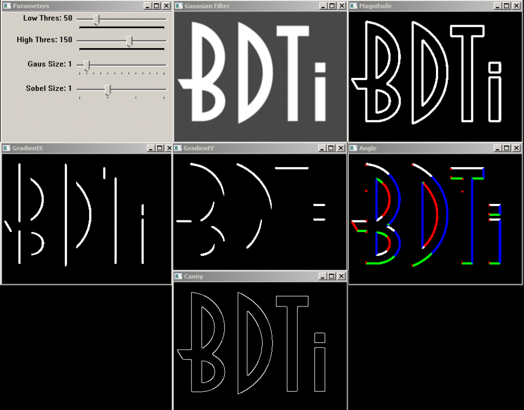
The edge detection demo included in the BDTI Quick-Start OpenCV Kit is shown in Figure 12 below.
Figure 12. OpenCV Canny example showing the edge detection process
The demo software can process a static image, a video file, or the video stream from a web camera. Processing occurs in real-time so you see results on the fly. The demo opens multiple windows, representing various stages in Canny edge detection algorithm. All windows are updated in real-time. The next section describes each of the windows displayed by this demo.
Canny Edge Detector Example Window Names and Functions
Parameters: Allows you to modify the Canny parameters on the fly using simple slider controls.
The parameters controlled by the sliders are:
Low Thres: Canny Low Threshold Parameter (T2) (LowThres)
High Thres: Canny High Threshold Parameter (T1) (HighThres)
Gaus Size: Gaussian Filter Size (Fsize)
Sobel Size: Sobel Operator Size (Ksize)
The corresponding OpenCV calls are:
// smooth gray scale image using Gaussian, output to image (blurred)
GaussianBlur( gray, blurred, Size(Fsize, Fsize), 0 );
// Perform Canny edge detection on image (blurred), output edgemap to (CannyEdges)
Canny( blurred, CannyEdges, LowThres, HighThres, Ksize );
Gaussian Filter: The output of the Gaussian filter.
GradientX: The result of the horizontal derivative (Sobel) of the image in the Gaussian Filter window.
GradientY: The result of the vertical derivative (Sobel) of the image in the Gaussian Filter window.
Magnitude: The result of combining the GradientX and GradientY images using the equation G = |Gx|+|Gy|
Angle: Color-coded result of the angle equation from Figure 8 combining GradientX and GradientY using arctan(Gy/Gx).
Black = 0 degrees
Red = 1 degree to 45 degrees
White = 46 degrees to 135 degrees
Blue = 136 degrees to 225 degrees
Green = 226 degrees to 315 degrees
Red = 316 degrees to 359 degrees
The 0-degree marker indicates the left to right direction, as shown in Figure 13 below.
Figure 13. The direction color code for the angle window in the Canny edge detector example. Left to right is 0 degrees
Canny: The Canny edgemap.
Conclusion
Edge detection is a fundamental building block in many computer vision and embedded vision applications. Edges represent unique groups of pixels that form natural boundaries around objects. By robustly identifying edges, many vision applications make an important first step towards discerning meaning from images.
Edges can be used to separate the objects in an image, in an operation referred to as segmentation. The output of an edge detector is called an edge map. In an edge map, pixels represent the edges detected in the original image. Edge maps find use by subsequent algorithms to group and classify objects.
The Canny algorithm is an optimal algorithm (per Canny’s criteria) for finding edges in a grayscale image. The algorithm produces thin edges that are well localized, accurately indicating the position of the edge in the image. Canny is a multi-stage algorithm, but only two lines of code are required to invoke it in OpenCV.
BDTI has created two tools to help engineers get started in computer vision quickly. The Windows-based BDTI OpenCV Executable Demo Package allows you to experiment with OpenCV algorithms such as edge detection, face detection, line detection, optical flow and Canny edge detection. It requires no programming; the demos can be run with the click of a mouse.
The BDTI Quick-Start OpenCV Kit is a VMware virtual machine image with OpenCV pre-installed, along with all required tools. The kit contains the same examples as in the BDTI OpenCV Executable Demo Package, along with full source code. The BDTI Quick-Start OpenCV Kit is intended for developers who want to quickly get started using OpenCV for computer vision application development. Simply modify the provided examples to begin implementing your own algorithm ideas.
Eric Gregori is a Senior Software Engineer and Embedded Vision Specialist with Berkeley Design Technology, Inc. (BDTI), which provides analysis, advice, and engineering for embedded processing technology and applications. He is a robot enthusiast with over 17 years of embedded firmware design experience, with specialties in computer vision, artificial intelligence, and programming for Windows Embedded CE, Linux, and Android operating systems.
To read more about the topic of embedded vision, go to “Jumping on the embedded vision bandwagon.”
(Editor’s Note: The Embedded Vision Alliance was launched in May of 2011, and now has 19 sponsoring member companies: AMD, Analog Devices, Apical, Avnet Electronics Marketing, BDTI, CEVA, Cognimem, CogniVue, eyeSight, Freescale, IMS Research, Intel, MathWorks, Maxim Integrated Products, NVIDIA, National Instruments, Omek Interactive, Texas Instruments, Tokyo Electron Device, and Xilinx.
The first step of the Embedded Vision Alliance was to launch a website at www.Embedded-Vision.com. The site serves as a source of practical information to help design engineers and application developers incorporate vision capabilities into their products. The Alliance’s plans include educational webinars, industry reports, and other related activities.
Everyone is free to access the resources on the website, which is maintained through member and industry contributions. Membership details are also available at the site. For more information, contact the Embedded Vision Alliance at [email protected] and 1-510-451-1800.)

