Using Convolutional Neural Networks for Image Recognition

This article was originally published at Cadence's website. It is reprinted here with the permission of Cadence.

Convolutional neural networks (CNNs) are widely used in pattern- and image-recognition problems as they have a number of advantages compared to other techniques. This white paper covers the basics of CNNs including a description of the various layers used. Using traffic sign recognition as an example, we discuss the challenges of the general problem and introduce algorithms and implementation software developed by Cadence that can trade off computational burden and energy for a modest degradation in sign recognition rates. We outline the challenges of using CNNs in embedded systems and introduce the key characteristics of the Cadence® Tensilica® Vision P5 digital signal processor (DSP) for Imaging and Computer Vision and software that make it so suitable for CNN applications across many imaging and related recognition tasks.

What Is a CNN?

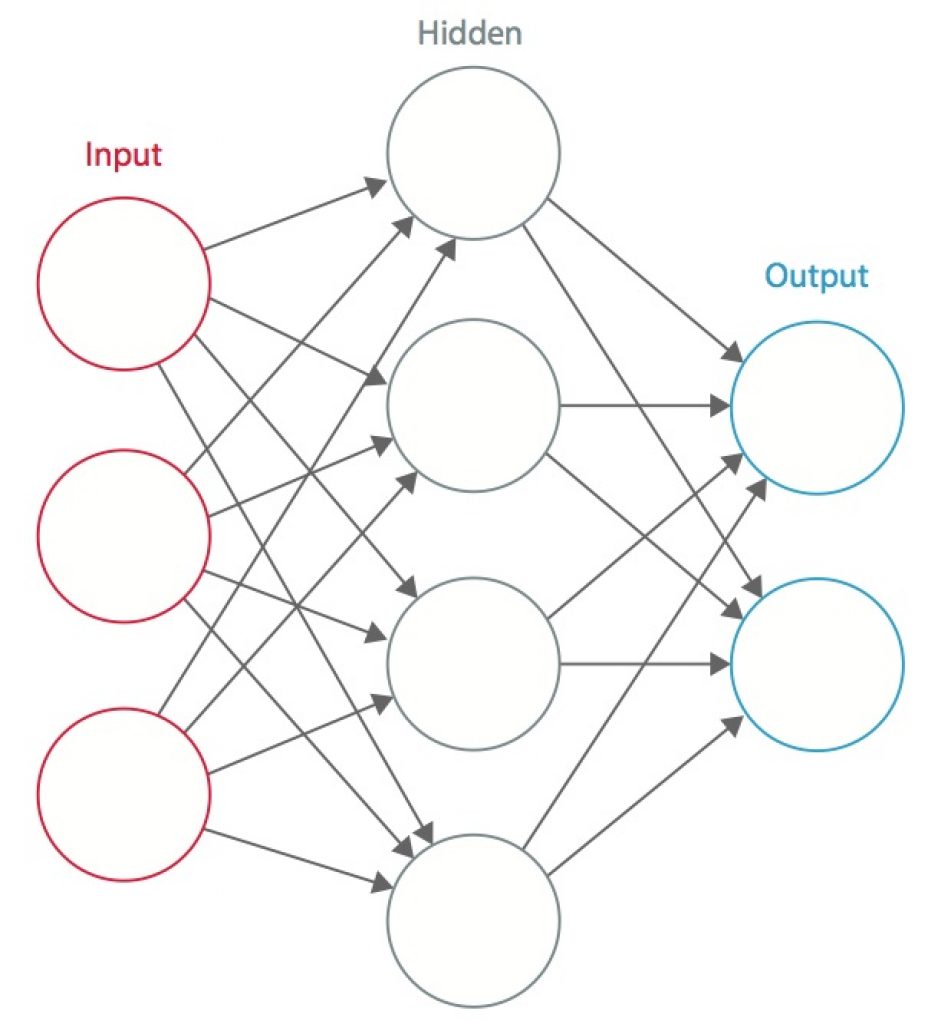
A neural network is a system of interconnected artificial “neurons” that exchange messages between each other. The connections have numeric weights that are tuned during the training process, so that a properly trained network will respond correctly when presented with an image or pattern to recognize. The network consists of multiple layers of feature-detecting “neurons”. Each layer has many neurons that respond to different combinations of inputs from the previous layers. As shown in Figure 1, the layers are built up so that the first layer detects a set of primitive patterns in the input, the second layer detects patterns of patterns, the third layer detects patterns of those patterns, and so on. Typical CNNs use 5 to 25 distinct layers of pattern recognition.

Figure 1: An artificial neural network [1]

Training is performed using a “labeled” dataset of inputs in a wide assortment of representative input patterns that are tagged with their intended output response. Training uses general-purpose methods to iteratively determine the weights for intermediate and final feature neurons. Figure 2 demonstrates the training process at a block level.

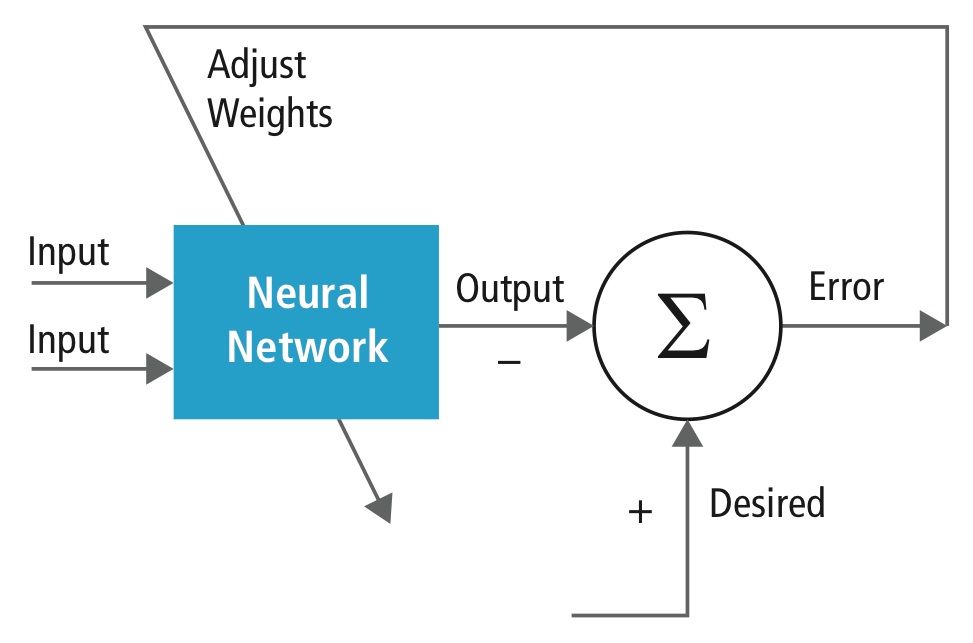
Figure 2: Training of neural networks

Neural networks are inspired by biological neural systems. The basic computational unit of the brain is a neuron and they are connected with synapses. Figure 3 compares a biological neuron with a basic mathematical model [2].

Figure 3: Illustration of a biological neuron (top) and its mathematical model (bottom) [2]

In a real animal neural system, a neuron is perceived to be receiving input signals from its dendrites and producing output signals along its axon. The axon branches out and connects via synapses to dendrites of other neurons. When the combination of input signals reaches some threshold condition among its input dendrites, the neuron is triggered and its activation is communicated to successor neurons.

In the neural network computational model, the signals that travel along the axons (e.g., x₀) interact multiplicatively (e.g., w₀x₀) with the dendrites of the other neuron based on the synaptic strength at that synapse (e.g., w₀). Synaptic weights are learnable and control the influence of one neuron or another. The dendrites carry the signal to the cell body, where they all are summed. If the final sum is above a specified threshold, the neuron fires, sending a spike along its axon. In the computational model, it is assumed that the precise timings of the firing do not matter and only the frequency of the firing communicates information. Based on the rate code interpretation, the firing rate of the neuron is modeled with an activation function ƒ that represents the frequency of the spikes along the axon. A common choice of activation function is sigmoid. In summary, each neuron calculates the dot product of inputs and weights, adds the bias, and applies non-linearity as a trigger function (for example, following a sigmoid response function).

A CNN is a special case of the neural network described above. A CNN consists of one or more convolutional layers, often with a subsampling layer, which are followed by one or more fully connected layers as in a standard neural network.

The design of a CNN is motivated by the discovery of a visual mechanism, the visual cortex, in the brain. The visual cortex contains a lot of cells that are responsible for detecting light in small, overlapping sub-regions of the visual field, which are called receptive fields. These cells act as local filters over the input space, and the more complex cells have larger receptive fields. The convolution layer in a CNN performs the function that is performed by the cells in the visual cortex [3].

A typical CNN for recognizing traffic signs is shown in Figure 4. Each feature of a layer receives inputs from a set of features located in a small neighborhood in the previous layer called a local receptive field. With local receptive fields, features can extract elementary visual features, such as oriented edges, end-points, corners, etc., which are then combined by the higher layers.

In the traditional model of pattern/image recognition, a hand-designed feature extractor gathers relevant infor- mation from the input and eliminates irrelevant variabilities. The extractor is followed by a trainable classifier, a standard neural network that classifies feature vectors into classes.

In a CNN, convolution layers play the role of feature extractor. But they are not hand designed. Convolution filter kernel weights are decided on as part of the training process. Convolutional layers are able to extract the local features because they restrict the receptive fields of the hidden layers to be local.

Figure 4: Typical block diagram of a CNN [4]

CNNs are used in variety of areas, including image and pattern recognition, speech recognition, natural language processing, and video analysis. There are a number of reasons that convolutional neural networks are becoming important. In traditional models for pattern recognition, feature extractors are hand designed. In CNNs, the weights of the convolutional layer being used for feature extraction as well as the fully connected layer being used for classification are determined during the training process. The improved network structures of CNNs lead to savings in memory requirements and computation complexity requirements and, at the same time, give better performance for applications where the input has local correlation (e.g., image and speech).

Large requirements of computational resources for training and evaluation of CNNs are sometimes met by graphic processing units (GPUs), DSPs, or other silicon architectures optimized for high throughput and low energy when executing the idiosyncratic patterns of CNN computation. In fact, advanced processors such as the Tensilica Vision P5 DSP for Imaging and Computer Vision from Cadence have an almost ideal set of computation and memory resources required for running CNNs at high efficiency.

In pattern and image recognition applications, the best possible correct detection rates (CDRs) have been achieved using CNNs. For example, CNNs have achieved a CDR of 99.77% using the MNIST database of handwritten digits [5], a CDR of 97.47% with the NORB dataset of 3D objects [6], and a CDR of 97.6% on ~5600 images of more than 10 objects [7]. CNNs not only give the best performance compared to other detection algorithms, they even outperform humans in cases such as classifying objects into fine-grained categories such as the particular breed of dog or species of bird [8].

Figure 5 shows a typical vision algorithm pipeline, which consists of four stages: pre-processing the image, detecting regions of interest (ROI) that contain likely objects, object recognition, and vision decision making. The pre-processing step is usually dependent on the details of the input, especially the camera system, and is often implemented in a hardwired unit outside the vision subsystem. The decision making at the end of pipeline typically operates on recognized objects—It may make complex decisions, but it operates on much less data, so these decisions are not usually computationally hard or memory-intensive problems. The big challenge is in the object detection and recognition stages, where CNNs are now having a wide impact.

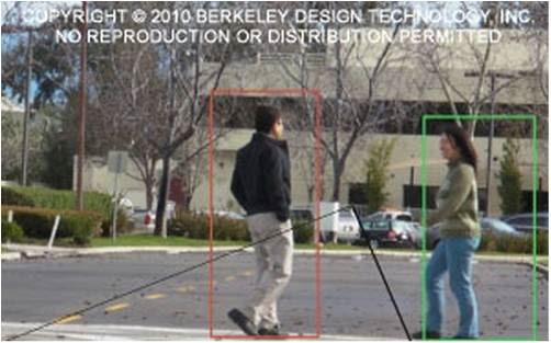
Figure 5: Vision algorithm pipeline

Layers of CNNs

By stacking multiple and different layers in a CNN, complex architectures are built for classification problems. Four types of layers are most common: convolution layers, pooling/subsampling layers, non-linear layers, and fully connected layers.

Convolution layers

The convolution operation extracts different features of the input. The first convolution layer extracts low-level features like edges, lines, and corners. Higher-level layers extract higher-level features. Figure 6 illustrates the process of 3D convolution used in CNNs. The input is of size N x N x D and is convolved with H kernels, each of
size k x k x D separately. Convolution of an input with one kernel produces one output feature, and with H kernels independently produces H features. Starting from top-left corner of the input, each kernel is moved from left to right, one element at a time. Once the top-right corner is reached, the kernel is moved one element in a downward direction, and again the kernel is moved from left to right, one element at a time. This process is repeated until
the kernel reaches the bottom-right corner. For the case when N = 32 and k = 5 , there are 28 unique positions from left to right and 28 unique positions from top to bottom that the kernel can take. Corresponding to these positions, each feature in the output will contain 28×28 (i.e., (N-k+1) x (N-k+1)) elements. For each position of the kernel in a sliding window process, k x k x D elements of input and k x k x D elements of kernel are element-by- element multiplied and accumulated. So to create one element of one output feature, k x k x D multiply-accumulate operations are required.

Figure 6: Pictorial representation of convolution process [9]

Pooling/subsampling layers

The pooling/subsampling layer reduces the resolution of the features. It makes the features robust against noise and distortion. There are two ways to do pooling: max pooling and average pooling. In both cases, the input is divided into non-overlapping two-dimensional spaces. For example, in Figure 4, layer 2 is the pooling layer. Each input feature is 28×28 and is divided into 14×14 regions of size 2×2. For average pooling, the average of the four values in the region are calculated. For max pooling, the maximum value of the four values is selected.

Figure 7 elaborates the pooling process further. The input is of size 4×4. For 2×2 subsampling, a 4×4 image is divided into four non-overlapping matrices of size 2×2. In the case of max pooling, the maximum value of the four values in the 2×2 matrix is the output. In case of average pooling, the average of the four values is the output. Please note that for the output with index (2,2), the result of averaging is a fraction that has been rounded to nearest integer.

Figure 7: Pictorial representation of max pooling and average pooling [3]

Non-linear layers

Neural networks in general and CNNs in particular rely on a non-linear “trigger” function to signal distinct identifi- cation of likely features on each hidden layer. CNNs may use a variety of specific functions —such as rectified linear units (ReLUs) and continuous trigger (non-linear) functions—to efficiently implement this non-linear triggering.

ReLU

A ReLU implements the function y = max(x,0), so the input and output sizes of this layer are the same. It increases the nonlinear properties of the decision function and of the overall network without affecting the receptive fields of the convolution layer. In comparison to the other non-linear functions used in CNNs (e.g., hyperbolic tangent, absolute of hyperbolic tangent, and sigmoid), the advantage of a ReLU is that the network trains many times faster. ReLU functionality is illustrated in Figure 8, with its transfer function plotted above the arrow.

Figure 8: Pictorial representation of ReLU functionality

Continuous trigger (non-linear) function

The non-linear layer operates element by element in each feature. A continuous trigger function can be hyperbolic tangent (Figure 9), absolute of hyperbolic tangent (Figure 10), or sigmoid (Figure 11). Figure 12 demonstrates how non-linearity gets applied element by element.

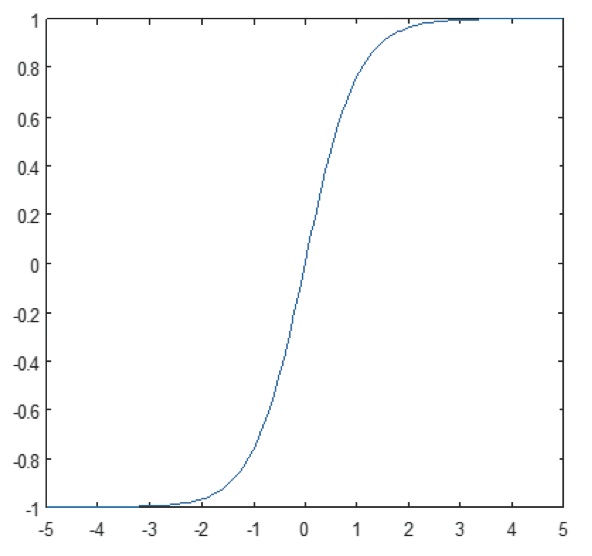
Figure 9: Plot of hyperbolic tangent function

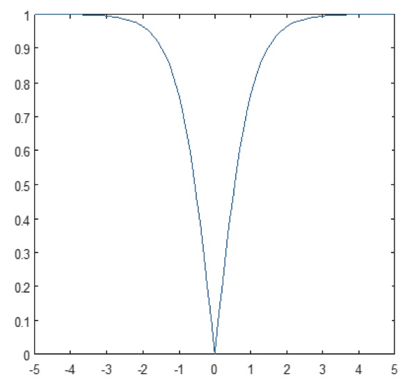
Figure 10: Plot of absolute of hyperbolic tangent function

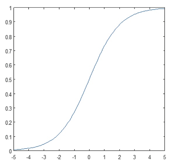
Figure 11: Plot of sigmoid function

Figure 12: Pictorial representation of tanh processing

Fully connected layers

Fully connected layers are often used as the final layers of a CNN. These layers mathematically sum a weighting of the previous layer of features, indicating the precise mix of “ingredients” to determine a specific target output result. In case of a fully connected layer, all the elements of all the features of the previous layer get used in the calculation of each element of each output feature.

Figure 13 explains the fully connected layer L. Layer L-1 has two features, each of which is 2×2, i.e., has four elements. Layer L has two features, each having a single element.

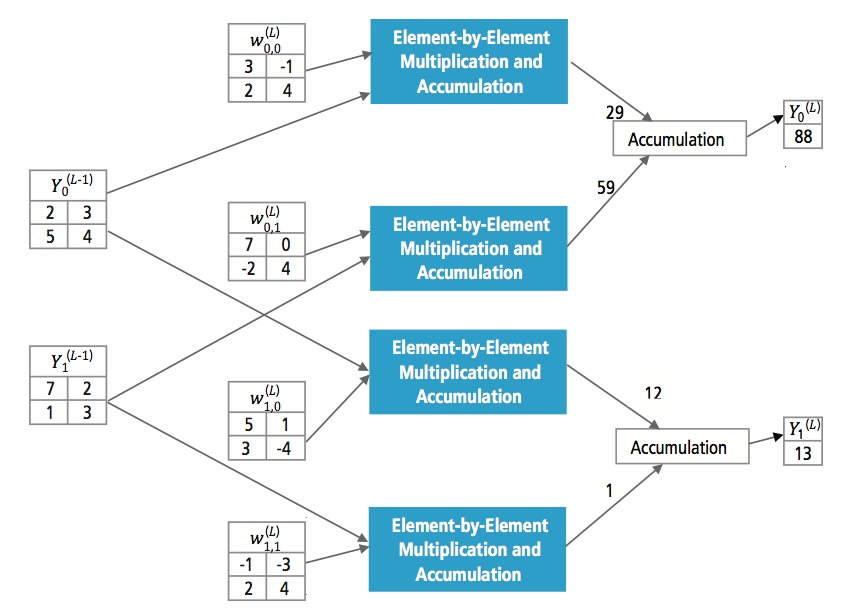
Figure 13: Processing of a fully connected layer

Why CNN?

While neural networks and other pattern detection methods have been around for the past 50 years, there has been significant development in the area of convolutional neural networks in the recent past. This section covers the advantages of using CNN for image recognition.

Ruggedness to shifts and distortion in the image

Detection using CNN is rugged to distortions such as change in shape due to camera lens, different lighting condi- tions, different poses, presence of partial occlusions, horizontal and vertical shifts, etc. However, CNNs are shift invariant since the same weight configuration is used across space. In theory, we also can achieve shift invari- antness using fully connected layers. But the outcome of training in this case is multiple units with identical weight patterns at different locations of the input. To learn these weight configurations, a large number of training instances would be required to cover the space of possible variations.

Fewer memory requirements

In this same hypothetical case where we use a fully connected layer to extract the features, the input image of size 32×32 and a hidden layer having 1000 features will require an order of 106 coefficients, a huge memory requirement. In the convolutional layer, the same coefficients are used across different locations in the space, so the memory requirement is drastically reduced.

Easier and better training

Again using the standard neural network that would be equivalent to a CNN, because the number of param- eters would be much higher, the training time would also increase proportionately. In a CNN, since the number of parameters is drastically reduced, training time is proportionately reduced. Also, assuming perfect training, we can design a standard neural network whose performance would be same as a CNN. But in practical training,
a standard neural network equivalent to CNN would have more parameters, which would lead to more noise addition during the training process. Hence, the performance of a standard neural network equivalent to a CNN will always be poorer.

Recognition Algorithm for GTSRB Dataset

The German Traffic Sign Recognition Benchmark (GTSRB) was a multi-class, single-image classification challenge held at the International Joint Conference on Neural Networks (IJCNN) 2011, with the following requirements:

• 51,840 images of German road signs in 43 classes (Figures 14 and 15)
• Size of images varies from 15×15 to 222×193
• Images are grouped by class and track with at least 30 images per track
• Images are available as color images (RGB), HOG features, Haar features, and color histograms
• Competition is only for the classification algorithm; algorithm to find region of interest in the frame is not required
• Temporal information of the test sequences is not shared, so temporal dimension cannot be used in the classification algorithm

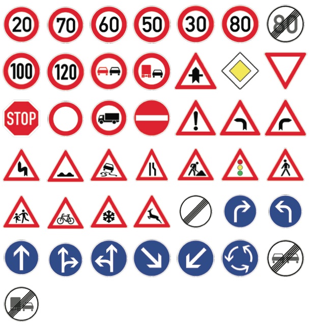
Figure 14: GTSRB ideal traffic signs

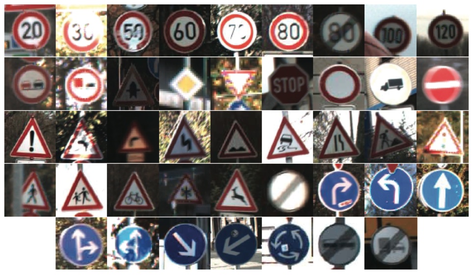
Figure 15: GTSRB traffic signs with impairments [10]

Cadence Algorithm for Traffic Sign Recognition in GTSRB Dataset

Cadence has developed various algorithms in MATLAB for traffic sign recognition using the GTSRB dataset, starting with a baseline configuration based on a well-known paper on sign recognition [1]. The correct detection rate of 99.24% and compute effort of almost >50 million multiply-adds per sign is shown as a thick green point in Figure 16. Cadence has achieved meaningfully better results using our new proprietary Hierarchical CNN approach. In this algorithm, 43 traffic signs have been divided into five families. In total, we implement six smaller CNNs. The first CNN decides which family the received traffic sign belongs to. Once the family of the sign is known, the CNN (one of the remaining five) corresponding to the family detected is run to decide the traffic sign within that family. Using this algorithm, Cadence has achieved a correct detection rate of 99.58%, the best CDR achieved on GTSRB to date.

Algorithm for Performance vs. Complexity Tradeoff

In order to control the complexity of CNNs in embedded applications, Cadence has also developed a proprietary algorithm using eigenvalue decomposition that reduces a trained CNN to its canonical dimension. Using this algorithm, we have been able to drastically reduce the complexity of the CNN without any performance degra- dation, or with a small controlled CDR reduction. Figure 16 shows the results achieved:

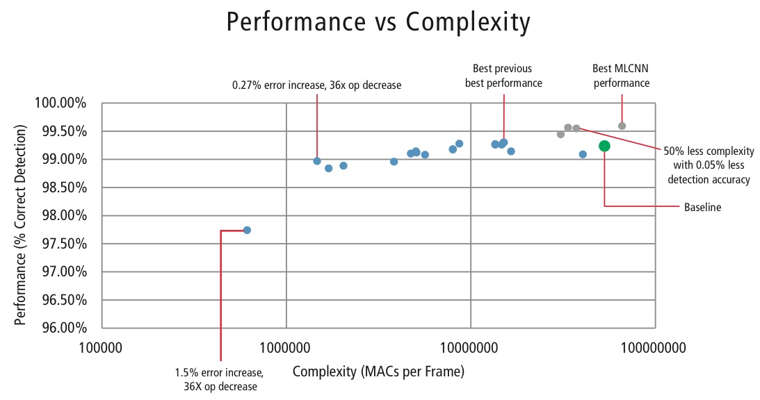
Figure 16: Performance vs. complexity plot for various CNN configurations to detect traffic signs in GTSRB dataset

The green point in Figure 16 is the baseline configuration. This configuration is quite close to the configuration suggested in Reference [4]. It requires 53 MMACs per frame for an error rate of 0.76%.

• The second point from the left requires 1.47 million MACs per frame for an error rate of 1.03%, i.e., for an increase in the error rate of 0.27%, the MAC requirement has been reduced by a factor of 36.14.
• The leftmost point requires 0.61 MMACs per frame for achieving an error rate of 2.26%, i.e., the number of MACs is reduced by a factor of 86.4 times.
• The points in blue are for a single-level CNN, whereas the points in red are for a hierarchical CNN. A best-case performance of 99.58% is achieved by the hierarchical CNN.

CNNs in Embedded Systems

As shown in Figure 5, a vision subsystem requires a lot of image processing in addition to a CNN. In order to run CNNs on a power-constrained embedded system that supports image processing, it should fulfill the following requirements:

• Availability of high computational performance: For a typical CNN implementation, billions of MACs per second is the requirement.
• Larger load/store bandwidth: In the case of a fully connected layer used for classification purpose, each coefficient gets used in multiplication only once. So, the load-store bandwidth requirement is greater than the number of MACs performed by the processor.
• Low dynamic power requirement: The system should consume less power. To address this issue, fixed-point implementation is required, which imposes the requirement of meeting the performance requirements using the minimum possible finite number of bits.
• Flexibility: It should be possible to easily upgrade the existing design to new better performing design.

Since computational resources are always a constraint in embedded systems, if the use case allows a small degra- dation in performance, it is helpful to have an algorithm that can achieve huge savings in computational complexity at the cost of a controlled small degradation in performance. So, Cadence’s work on an algorithm to achieve complexity versus a performance tradeoff, as explained in the previous section, has great relevance for imple- menting CNNs on embedded systems.

CNNs on Tensilica Processors

The Tensilica Vision P5 DSP is a high-performance, low-power DSP specifically designed for image and computer vision processing. The DSP has a VLIW architecture with SIMD support. It has five issue slots in an instruction word of up to 96 bits and can load up to 1024-bit words from memory every cycle. Internal registers and operation units range from 512 bits to 1536 bits, where the data is represented as 16, 32, or 64 slices of 8b, 16b, 24b, 32b, or 48b pixel data.

The DSP addresses all the challenges for implementing CNNs in embedded systems as discussed in the previous section.

• Availability of high computational performance: In addition to the advanced support for implementing image signal processing, the DSP has instruction support for all stages of CNNs. For convolution operations, it has a very rich instruction set supporting multiply/multiply-accumulate operations supporting 8b x 8b, 8b x 16b and 16b x 16b operations for signed/unsigned data. It can perform up to 64 8b x 16b and 8b x 8b multiply/multiply- accumulate operations in one cycle and 32 16b x 16b multiply/multiply-accumulate operations in one cycle. For max pooling and ReLU functionality, the DSP has instructions to do 64 8-bit comparisons in one cycle. For implementing non-linear functions with finite ranges like tanh and signum, it has instructions to implement a look-up table for 64 7-bit values in one cycle. In most of the cases, instructions for comparison and look-up table get scheduled in parallel with multiply/multiply-accumulate instructions and do not take any extra cycles.
• Larger load/store bandwidth: The DSP can perform up to two 512-bit load/store operations per cycle.
• Low dynamic power requirement: The DSP is a fixed-point machine. Due to the flexible handling of a variety of data types, full performance and energy advantage of mixed 16b and 8b computation can be achieved at minimal loss of accuracy.
• Flexibility: Since the DSP is a programmable processor, the system can be upgraded to a new version just by performing a firmware upgrade.
• Floating Point: For algorithms requiring an extended dynamic range for their data and/or coefficients, the DSP has an optional vector floating-point unit.

The Vision P5 DSP is delivered with a complete set of software tools that includes a high-performance C/C++ compiler with automatic vectorization and scheduling to support the SIMD and VLIW architecture without the need to write assembly language. This comprehensive toolset also includes the linker, assembler, debugger, profiler, and graphical visualization tools. A comprehensive instruction set simulator (ISS) allows the designer to quickly simulate and evaluate performance. When working with large systems or lengthy test vectors, the fast, functional TurboXim simulator option achieves speeds that are 40X to 80X faster than the ISS for efficient software development and functional verification.

Cadence has implemented a single-layer architecture CNN on the DSP for German traffic sign recognition. Cadence has achieved a CDR of 99.403% with 16-bit quantization for data samples and 8-bit quantization for coefficients in all the layers for this architecture. It has two convolution layers, three fully connected layers, four ReLU layers, three max pooling layers, and one tanh non-linear layer. Cadence has achieved a performance of 38.58 MACs/ cycle on an average for the complete network including the cycles for all the max pooling, tanh, and ReLU layers. Cadence has achieved best-case performance of 58.43 MACs per cycle for the third layer, including the cycles for tanh and ReLU functionalities. This DSP running at 600MHz can process more than 850 traffic signs in one second.

The Future of CNNs

Among the promising areas of neural networks research are recurrent neural networks (RNNs) using long short- term memory (LSTM). These areas are delivering the current state of the art in time-series recognition tasks like speech recognition and handwriting recognition. RNN/autoencoders are also capable of generating handwriting/ speech/images with some known distribution [10],[11],[12],[13],[14].

Deep belief networks, another promising type of network utilizing restricted Boltzman machines (RMBs)/autoen- coders, are capable of being trained greedily, one layer at a time, and hence are more easily trainable for very deep networks [15],[16].

Conclusion

CNNs give the best performance in pattern/image recognition problems and even outperform humans in certain cases. Cadence has achieved best-in-industry results using proprietary algorithms and architectures with CNNs. We have developed hierarchical CNNs for recognizing traffic signs in the GTSRB, achieving the best performance ever on this dataset. We have developed another algorithm for the performance-versus-complexity tradeoff and have been able to achieve a complexity reduction by a factor of 86 for a CDR degradation of less than 2%. The Tensilica Vision P5 DSP for imaging and computer vision from Cadence has all the features required to implement CNNs in addition to the features required to do image signal processing. More than 850 traffic sign recognitions can be performed running the DSP at 600MHz. The Tensilica Vision P5 DSP from Cadence has an almost ideal set of features to run CNNs.

References

[1] “Artificial neural network.” Wikipedia. https://en.wikipedia.org/wiki/Artificial_neural_network

[2] Karpathy, Andrej. 2015. “Neural Networks Part 1: Setting Up the Architecture.” Notes for CS231n Convolutional Neural Networks for Visual Recognition, Stanford University. http://cs231n.github.io/neural-networks-1/

[3] “Convolutional neural network.” Wikipedia. https://en.wikipedia.org/wiki/Convolutional_neural_network

[4] Sermanet, Pierre, and Yann LeCun. 2011. “Traffic Sign Recognition with Multi Scale Networks.” Courant Institute of Mathematical Sciences, New York University. http://ieeexplore.ieee.org/xpl/login.jsp?tp=&arnumber=6033589

[5] Ciresan, Dan, Ueli Meier, and Jürgen Schmidhuber. 2012. “Multi-column deep neural networks for image classi- fication.” 2012 IEEE Conference on Computer Vision and Pattern Recognition (New York, NY: Institute of Electrical and Electronics Engineers (IEEE)). http://ieeexplore.ieee.org/xpl/login.jsp?tp=&arnumber=6248110

[6] Ciresan, Dan, Ueli Meier, Jonathan Masci, Luca M. Gambardella, and Jurgen Schmidhuber. 2011. “Flexible, High Performance Convolutional Neural Networks for Image Classification.” Proceedings of the Twenty-Second International Joint Conference on Artificial Intelligence-Volume Two: 1237–1242. Retrieved 17 November 2013. http://people.idsia.ch/~juergen/ijcai2011.pdf

[7] Lawrence, Steve, C. Lee Giles, Ah Chung Tsoi, and Andrew D. Back. 1997. “Face Recognition: A Convolutional Neural Network Approach.” IEEE Transactions on Neural Networks, Volume 8; Issue 1. http://ieeexplore.ieee.org/xpl/login.jsp?tp=&arnumber=554195

[8] Russakovsky, O. et al. 2014. “ImageNet Large Scale Visual Recognition Challenge.” International Journal of Computer Vision. http://link.springer.com/article/10.1007/s11263-015-0816-y#

[9] Ovtcharov, Kalin, Olatunji Ruwarse, Joo-Young Kim et al. Feb 22, 2015. “Accelerating Deep Convolutional Networks Using Specialized Hardware.” Microsoft Research. http://research-srv.microsoft.com/pubs/240715/CNN%20Whitepaper.pdf

[10] Stallkamp, J., M. Schlipsing, J. Salmen, and C. Igel. “Man Vs. Computer: Benchmarking Machine Learning Algorithms For Traffic Sign Application.” IJCNN 2011. http://www.sciencedirect.com/science/article/pii/S0893608012000457

[11] Hochreiter, Sepp, and Jürgen Schmidhuber. 1997. “Long Short-Term Memory.” Neural Computation, 9(8):1735–1780. ftp://ftp.idsia.ch/pub/juergen/lstm.pdf

[12] Graves, Alex. 2014. “Generating Sequences With Recurrent Neural Networks.” http://arxiv.org/abs/1308.0850

[13] Schmidhuber, Jurgen. 2015. “Recurrent Neural Networks.” http://people.idsia.ch/~juergen/rnn.html

[14] Olshausen, Bruno A., and David J. Field. 1996. “Emergence of simple-cell receptive field properties by learning a sparse code for natural images.” Nature 381.6583: 607-609. http://www.nature.com/nature/journal/v381/n6583/abs/381607a0.html

[15] Hinton, G. E. and Salakhutdinov, R. R. 2006. “Reducing the dimensionality of data with neural networks.” Science vol. 313 no. 5786 pp. 504-507. http://www.sciencemag.org/content/suppl/2006/08/04/313.5786.504.DC1.

[16] Hinton, Geoffrey E. 2009. “Deep belief networks.” Scholarpedia, 4(5):5947.
http://www.scholarpedia.org/article/Deep_belief_networks