This blog post was originally published at NVIDIA's website. It is reprinted here with the permission of NVIDIA.
Classification of astronomical sources in the night sky is important for understanding the universe. It helps us understand the properties of what makes up celestial systems, from our solar system to the most distant galaxy and everything in between. The Photometric LSST Astronomical Time-Series Classification Challenge (PLAsTiCC) wants to revolutionize the field by automatically classifying 10–100x faster than previous methods.
This will provide the open-source Kaggle data repository with a great new dataset to solve this partcular Kaggle problem using machine learning. I had the honor of representing RAPIDS.ai for this competition and ended up with 8th place out of 1094 teams! My solution achieved an up to 140x performance increase for ETL and 25x end-to-end speedup over the CPU solution. Here is the story of how we make sense of the universe in a RAPIDS way.
Background
Astronomers have spent centuries developing many ways to discern different types of stars, ranging from the naked human eyes to modern spectroscopic analysis methods. Spectroscopy takes light collected by modern telescopes and splits the light into individual wavelengths. This method extracts the exact fingerprint of the astrophysical sources by finding out what wavelengths are missing.
Unfortunately, this type of analysis requires substantial time, a problem exacerbated when trying to keep up with the enormous 40 Terabytes data per night data rate that the new Large Synoptic Survey Telescope (LSST) generates. Machine learning comes into play, learning the pattern from the light curves data directly. However, the vast amount of incoming data makes it difficult to ingest in real-time. The GPU becomes most promising solution to this problem, as my end-to-end GPU demo takes only 40 seconds to process 20 gigabytes of data!
This Kaggle challenge provides a training data set of 7000 objects and a test data set of 3 million objects. Each object consists of two types of information:
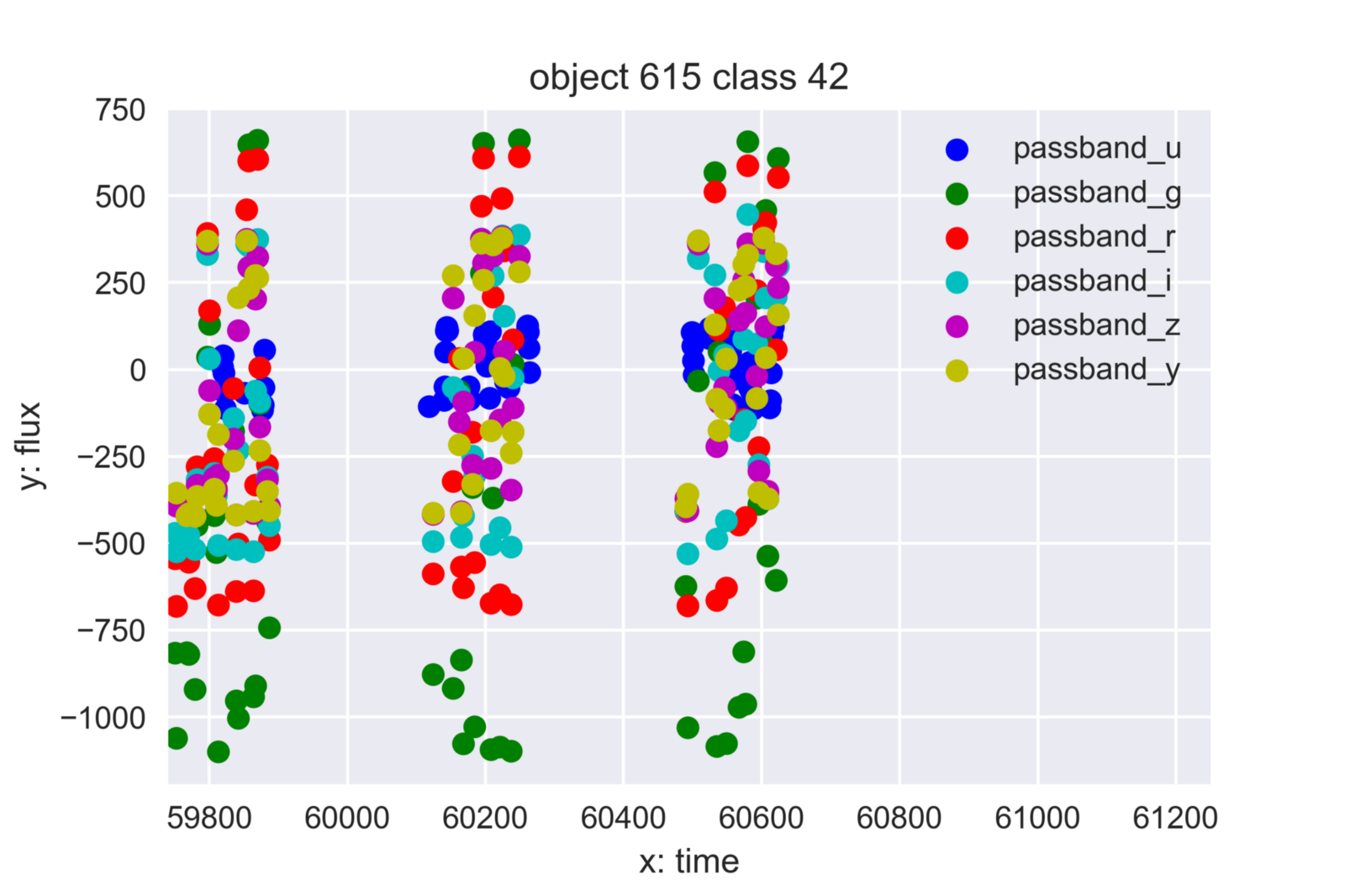
- Time series of observations of the objects, or so called light curves, shown in figure 1
- Meta features that do not vary over time.

Figure 1: The light curve time series by LSST of object 615 with all six passbands.
The light curve time series is the most critical information for solving the puzzle. Some common challenges with time series classification exist, such as:
- The length of light curve for each object could be very different. In this data set, it ranges from 100 to 500 observations. The light curve maps to a vector of a fixed dimensionality via two methods: cudf groupby aggregation and an RNN encoder.
- The brightness magnitude (flux) can have huge variance. Thus, logarithmic normalization becomes critical for neural network models.
Solution Overview
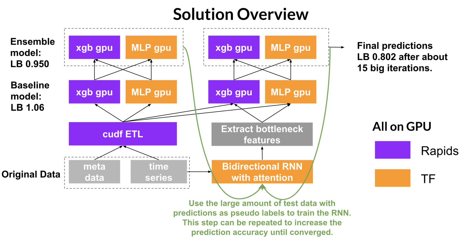
An all-GPU solution is implemented with Rapids.ai libraries and tensorflow, as diagrammed in figure 2.

Figure 2. Solution diagram based on Rapids and TensorFlow
Let’s walk through the steps required for this solution.
- Extract features from both time series and meta data using rapids cudf, especially the groupby aggregation functionality.
- Train base classifiers of Xgboost and multi-layer perceptron (MLP) with features from Step 1.
- Use predictions from Step 2 as features and train stack models.
- Use the predictions of test data from step 3 as pseudo labels to train a bidirectional recurrent neural network (RNN) and extract the bottleneck features with attention (the weighted sum of all hidden states of RNN cells).
- Use the bottleneck features of step 4 along with features from step 1 to train Xgboost and MLP again.
- Use predictions from step 5 as features and train stack models to get final predictions.
- Repeat steps 1 to 6 until the hold out validation accuracy converges.
Feature Engineering
RAPIDS’ cudf is crucial to efficient feature engineering and feature selection thanks to its accelerated performance using GPUs. The main features include statistical metrics (mean, max, etc) that summarize each object’s light curve characteristics with the groupby-aggregation operation. The input data is a dataframe with light curves of all the objects. The groupby-aggregation operation splits the dataframe based on the object ID, processes each object’s light curve independently and combines the summarized results back to one dataframe, which is ready for the classifier.
The GPU-based cudf achieves significant performance increases compared to the CPU based pandas. In general, the GPU-based cudf is at least 10x faster for reading data and groupby aggregation. In best case situations, groupby and aggregation with skewfunction, cudf achieves 120x~140x speedup. Although the skew function is not directly supportedy by cudf, I implemented a workaround with cudf’s apply_grouped primitives and numba to write GPU kernel functions, as shown in the code snippet below.
@cuda.jit(device=True)
def compute_skew_with_mean(array,skew,mean):
# skew is a shared memory array
# mean is a scaler, the mean value of array
# len(skew) == TPB+1
# TPB: constant, threads per block, 32 in this case
# the kernel has only one thread block, so no global sync required.
# the final result is in skew[0]
tid = cuda.threadIdx.x
initialize(skew,0,len(skew))
cuda.syncthreads()
tid = cuda.threadIdx.x
for i in range(cuda.threadIdx.x, len(array), cuda.blockDim.x):
skew[tid] += (array[i]-mean)**2
cuda.syncthreads()
reduction_sum(skew)
if tid == 0:
skew[TPB] = skew[0]/(len(array))
cuda.syncthreads()
initialize(skew,0,TPB)
cuda.syncthreads()
for i in range(cuda.threadIdx.x, len(array), cuda.blockDim.x):
skew[tid] += (array[i]-mean)**3
cuda.syncthreads()
reduction_sum(skew)
if tid == 0:
n = len(array)
m3 = skew[0]/(len(array)) # 3rd moment
m2 = skew[TPB] # 2nd moment
if m2>0 and n>2:
skew[0] = math.sqrt((n-1.0)*n)/(n-2.0)*m3/m2**1.5
else:
skew[0] = 0
cuda.syncthreads()
The speedup brought by RAPIDS is the key to ingesting the enormous data generated by LSST in real-time. These performance improvements increase data scientists’ efficiency, allowing fast iterative experimenting of ETL, feature selection, and practically every step of the machine learning pipeline. Eventually, these features feed to a GPU version of the Xgboost classifier, which already achieves 80% accuracy of the final complex ensemble.
Stacking and self-training.
The solid feature engineering allowed me to several good base models that placed in top 10% of the competition. Breaking into top 1% required employing some of the most effective kaggle tricks such as stacking and semi-supervised self-training.
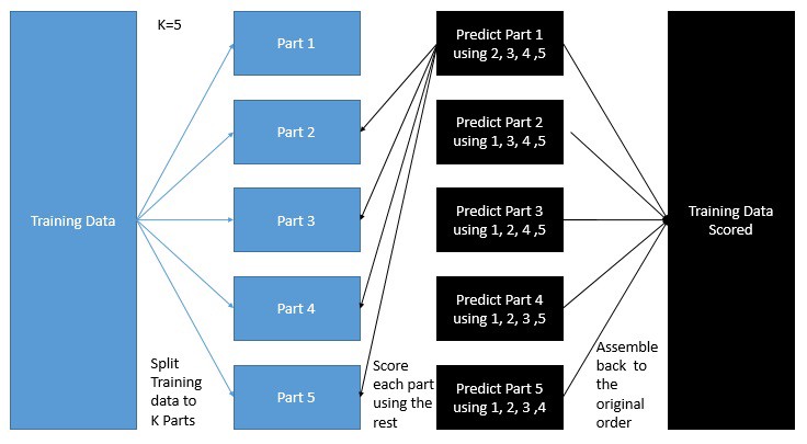
Stacking is a non-linear ensemble technique where new features are generated from the base models’ predictions in a cross validation manner, as shown in figure 3.

Figure 3. Model prediction cross-validation. (Image from Kazanova’s stacknet blog)
Self-training is a semi-supervised technique where predictions are used as pseudo labels. Different from stacking, self-training can train the unlabelled test data with pseudo labels, which essentially augment the training data. In this competition, the size of test data is 500x training data, so self-training can be very effective. Specifically, I built a bidirectional RNN to learn from the raw light curve time series directly with self-training.
This complements the manually-crafted features by cudf. Training the RNN uses all the test data while validation and early stopping uses only the original training data. In this way, we enforce the RNN to learn a middle ground that can fit the pseudo labels of test data and true labels of training data simultaneously. The loop of feature engineering, stacking, and self-training repeats until the holdout validation accuracy converges. More details about stacking and self-training can be found at my kaggle post.
Further improvement
Rapids is so fast and powerful that it’s easy to forget that it only arrived three months ago. As new as it is, Rapids offers great potential. Valuable lessons learned from the competition will enable us to improve Rapids. These include:
- Better GPU memory management. The main challenge of this competition is to handle the big data size. With a single GPU, out-of-memory error (OOM) is very likely to occur. To prevent such OOM errors, several tricks are utilized such as manually moving data back and forth between host and device, deleting columns immediately after operations and so on. Despite being effective and relatively low-overhead, such tricks still burden users with hardware details. Instead, we are working on dask-cudfintegration where large dataframes can be transparently ingested and manipulated in an out-of-core chunked manner.
- More functionalities. Kaggle competitions are all about distilling the last bit of useful information from data to push the accuracy. Hence kagglers crave every possible functions to transform the data from a different angle. For example, groupby-aggregation is the most common ETL trick which summarizes a group’s behavior by calculating a certain statistical metric. Currently some aggregation functions are not supported yet by rapids such as median. Workarounds for these functions can be implemented with cudf’s apply_grouped primitives and numba but there are definitely room for improvement.
- Consistency, readability, and everything else. Sometimes so much time can be saved from digging in the documents if the functions have consistent patterns and the error messages are straightforward. For example, most of the cudf’s functions return a dataframe or data series except for drop_column and reset_index, which are in place by default. We can either make them consistent or help users realize the difference with better naming of the functions or better error message.
Conclusion
This competition has been a fantastic learning process. Even with no astronomical background, I achieved amazing results through systematic iterative trial and error. None of these results would have been possible without the lightspeed rapids.ai library. If you want to learn more about how I built this application, feel free to take a look at the annotated source code. This reminds me why I love machine learning in the first place: with enough data, the right library, and massive computing power, the model can be (almost) as good as any domain experts.
Jiwei Liu
Data Scientist, NVIDIA


