This blog post was originally published at Syntiant’s website. It is reprinted here with the permission of Syntiant.
In our last blog post, we gave insight for modelers into the vital performance statistics of edge silicon. In this blog post, we will show how modelers can leverage the true power and throughput performance of edge neural accelerators to get the best task performance.
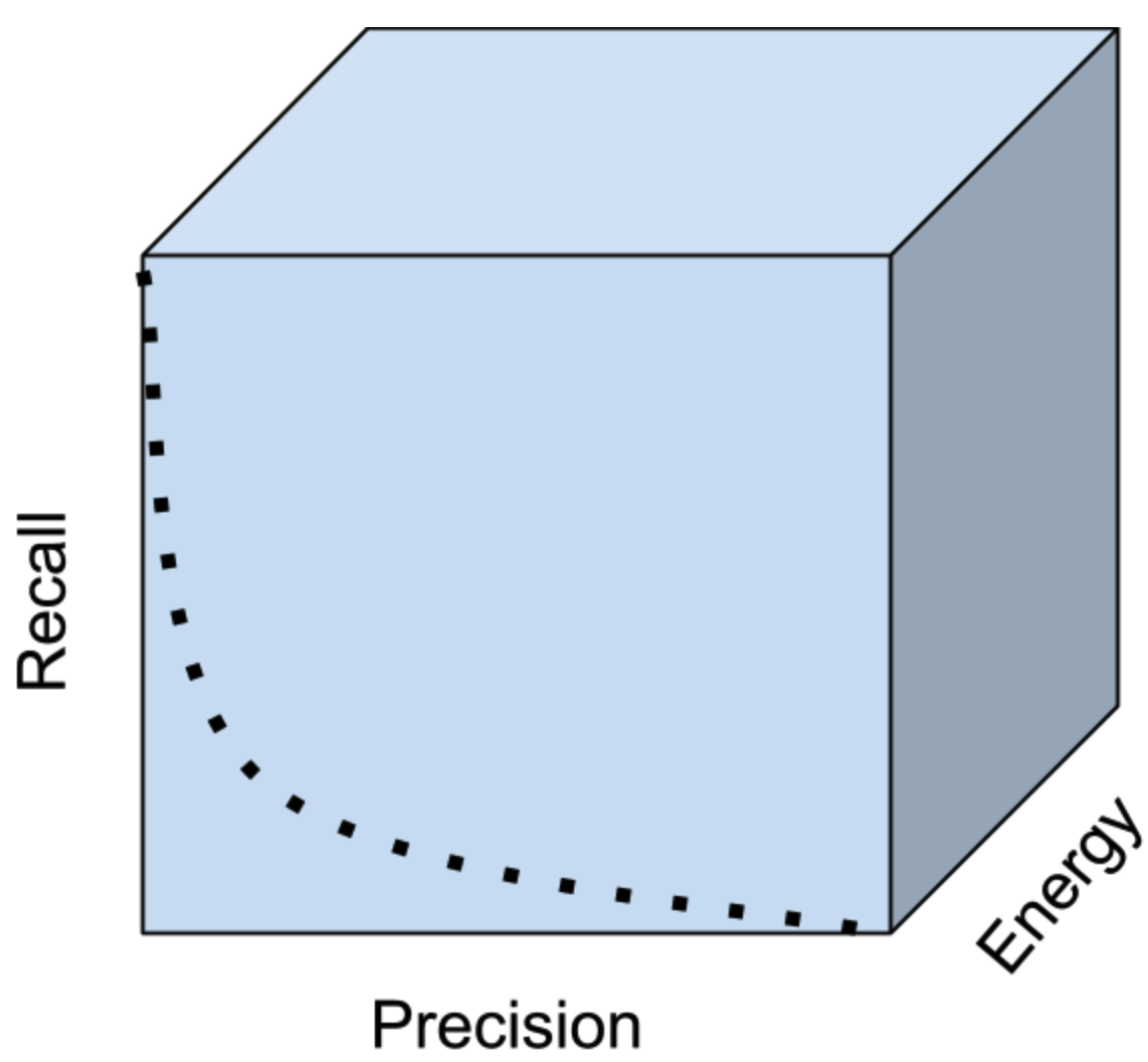
Machine learning researchers are familiar with the tension between precision and recall (the ability to correctly identify events, while detecting the events when they appear). Jointly optimizing a model to perform well by both these measures is a common modeling task, but battery-powered model deployments add inference energy as another attribute in tension with precision and recall. As modelers, optimizing three expensive output variables in tension (i.e., the post-training network performance) can be a nightmare. Thankfully, there are useful heuristics and design principles guiding you to strong compromise points between precision, recall, and energy.

Figure 1. Energy spent on inference is a hidden performance dimension determining achievable performance of machine learned systems. This blog post presumes an inference runtime has a power model allowing machine learning architects to explore the tradeoff space between solution attributes without running power measurements in a lab.
Let’s learn by example. Consider the two model architecture options below for a person detection computer vision task:
Option A. Use a big network 1 time per second
Option B. Use a 10x smaller version of the network 10 times per second
To a first-order, both options have the same average power, but which one should have the best performance and recall curve? Clearly option B provides 10x more time resolution on events with shorter latencies and the ability to localize events in time more accurately, but option A will have the strongest classification performance. When considering the solution in-context on a camera processing an infinite stream of images, these distinct performance properties tend to blend together. Every frame will be slightly different and people remain in view for multiple time steps. Leveraging the properties of the time series allows for increasing confidence in classifications by requiring multiple confirmations. In reality, you should not choose between the two options. You should frequently run a small model (Option B) and conditionally run the large model (Option A).
An age-old heuristic in energy efficient system design affirms this pattern: only run what you need to, when you need to. Here a system can run a small network that prioritizes recall (letting all candidate events through) while sacrificing precision. As long as the first network is reasonably selective, most of the energy is spent by the energy efficient first network. The critical step is to selectively run a more powerful secondary network to act as the final high-energy decision maker.
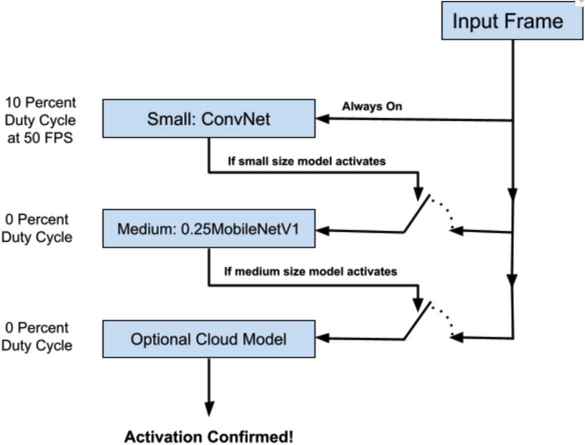
Let’s move from the abstract to the specific with a set of 3 architectures connected together as shown in Figure 2.

Figure 2: Cascading multiple models in a hypothetical person detection security camera running models on the NDP200. The small model is a relatively small convnet calibrated to high recall. The medium model is a quarter scale MobileNetV1 as configured by Google.
There is a lot of industry knowledge embedded in this solution design you will not find in machine learning conference proceedings, so let’s go into the details on “why” we have selected these 3 architecture configurations. When the small model is running, its NDP200 duty cycle is 10.3 percent. This means the network could run more than 9 times more often than it is configured to run for person detection. However, whenever the small model believes the target class is present, it switches to running a “medium model” until it either hands off to the cloud model or returns back to the small model. Since the high utilization runs conditionally, the exceedingly low duty cycle of the medium model (effectively zero) means it does not have a large impact on the power performance.
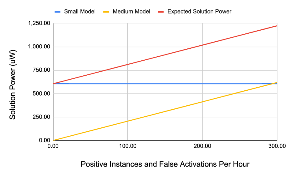
When might we want to configure this cascade differently? Figure 3 illustrates the tradeoff space according to the frequency of the target event. In low power solution design, a principle is to spend an equal amount of power on each stage of a cascade. If we expect to see 300 positive instances and false activations an hour, we have calibrated the relative model sizes properly. If however, the positive instances are far more common, then we should consider running a larger first stage model and potentially collapse the cascade.

Figure 3. Solution power for an increasing number of positive instances per hour. For rare event detection, the medium model has a minimal cost and could run as large as is supported by the hardware. For frequent events (i.e., after the medium model has higher solution power than the small model), then it is good to look at increasing the solution power of the small model.
These tradeoffs are challenging in nature because they involve hard choices balancing solution power, memory, latency, and user experience. You will not know the best path forward until you construct your starting cascade and begin iteratively optimizing your design. When selecting the environment within which you perform your architecture search, you can start by meeting your base requirements before optimizing in the duty cycle space. For instance, the small front-end model is configured to run 50 times per second. We could halve the power requirements by halving the frame rate. This is an example of a system parameter that is cheap to evaluate. Instead of performing computationally expensive training hyperparameter searches, you can run comparatively cheap parameter searches in the post-training space. Try sampling combinations of frame rates, stage confirmation requirements, and model precision/recall calibrations. All have massive effects on the duty cycling of edge neural accelerators
Rouzbeh Shirvani, Ph.D., and Sean McGregor, Ph.D.
Machine Learning Architects, Syntiant


